6. Processing description
This section gives a description of each step of the pipeline in a greater detail and list the parameters that can be changed if needed.
Next figure shows the main steps that are involved in the PANIC pipeline:
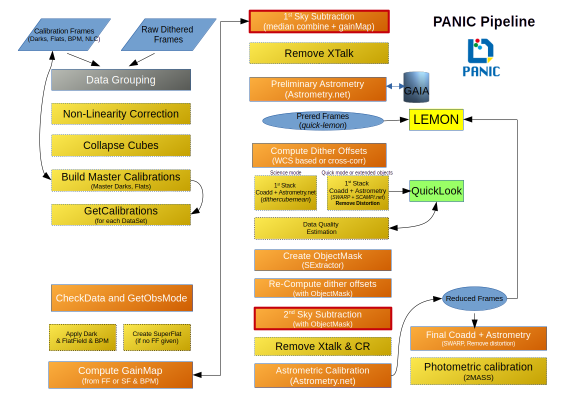
6.1. Outline
the non-linearity is corrected;
a master flat-field in computed by combining all the appropriate images without offsets; if the mosaic is of an Sky-Target type, only the sky frames are used;
a bad pixel mask, is computed by detecting, in the master flat field, the pixels with deviant values;
if provided, an external bad pixel mask is also used, adding the bad pixel in the previus one;
for each image, a sky frame is computed by combining a certain number of the closest images;
this sky frame is subtracted by the image and the result is divided by the master flat;
bright objects are detected by SExtractor in these cleaned images to measure the offsets among the images; the object mask are multiplied by the bad pixel mask to remove false detections;
a cross-correlation algorithm among the object masks is used to measure the relative offsets. It also works if no object is common to all the images;
the cleaned images are combined using the offsets, creating the “quick” image;
to remove the effect of faint obejcts on the estimate of the sky frames, SExtractor is used on the combined image to create a master object mask;
the object mask is dilatated by a certain factor to remove also the undetected object tails;
for each image a new sky is computed by taking into account this object mask;
if field distortion can be neglected, these images are combined by using the old offsets, creating the “science” image;
field distortion is removed from the cleaned images by using SCAMP computed distortion model
the pixels containing deviant pixels are identified and flagged;
the old offsets could be effected by field distortion, therefore new offsets are computed for the undistorted images;
finally, the cleaned corrected images are combined.
6.1.1. Main configuration file
See Main config file
6.1.2. Data-set classification
One of the main features of PAPI is that the software is able to do an automatic data reduction. While most of the pipelines are run interactively, PAPI is able to run without human interaction. It is done because of the classificaton algorithm that is implemented in PAPI and that allow an automatic identification of the data sets grouping the files according to the observation definition with the OT.
1 - The data grouping algorithm 2 - Sky finding algorithm for extended objects
In case of not using the OT during the observation, also a data grouping is possible, althouth with some limitations. Let’s see how it works:
[…]
6.1.3. Data Preparation
Firstly, each FITS file is linearity corrected if it was enabled in the configuration file (nonlinearity:apply). If integrations where done with repetitions >1 and saved as a cube with N-planes, then the FITS cube is collapsed doing a simple arithmetich sum of N-planes.
Then the image is divided into the number of chips in the FPA (which constitutes 4 chips in a mosaic). From this step on, the pipeline works on individual chips rather than whole images, thereby enhancing the speed and enabling us to do multi-chip processing on multi CPUs.
6.1.4. Calibrations
In next sections we describe the main calibration to be done by PAPI.
6.2. Computing the master dark
The master dark is built doing a median combine of a set of darks files with the same exposure time.
It is done in calDark.py module.
6.3. Computing the master flat-field
The master flat-field can be built from dome flat or sky (dusk or dawn) flats fields.
6.4. Computing the Bad Pixel Mask
The map of all bad pixels (hot, low QE) are derived from the non-linearity tests. However, also the nonlinearity analysis provides a list of non-correctable pixels, which always will be considered invalid.
So, currently there is no procedure in PAPI to compute the right bad pixel mask (BPM).
6.4.1. First pass sky subtraction
6.5. Sky model
In near-infrared (NIR) image processing, a sky model refers to an estimate of the spatial and temporal structure of the sky background emission, which is then subtracted from the science images. Constructing a good sky model is critical due to the bright, variable, and structured sky background in the NIR.
A good sky model should:
Capture temporal variation (via adjacent exposures or interpolation)
Preserve object flux (no over-subtraction)
Handle residual structures or instrumental effects (e.g. persistence, striping)
PAPI has implemented an sky model based on differenct strategies depending on the observing mode:
Using dithered target images.
For sparse fields or small targets, sky can be estimated from the science images themselves by dithering.
A sky model is built using a stack (median or sigma-clipped average) of temporally adjacent frames (2*hwidth), excluding the objects via masking.
This is known as a self-sky or sky from dither method.
Using dedicated sky frames.
When the target fills most of the field (e.g. extended objects), separate sky exposures (S) are taken.
A sky model is built by combining (e.g., median or sigma-clipped average) these temporally adjacent frames (2*hwidth) after masking sources.
The model is subtrated to each target frame. This is known as extended object method.
Fitting a sky surface per image.
A 2D surface or low-order polynomial is fitted to the background of each image after masking sources.
This local model is then subtracted. It is used for quick-look inspection of an target, and is kwnown as self-sky subtraction.
6.5.1. Object detection
The object detection is done using the well-known software SExtractor, using its most recent version.
6.5.2. Offset computation
TBD
6.5.3. First pass coaddition
TBD
6.5.4. Master object mask
SExtractor is again used to find objects in this first-pass coadded image in order to mask then during next sky estimation. This time the parameters controlling the detection threshold should be set to have deeper detections and mask faint objects. The parameters involved nad ther default values are:
mask_minarear = 10 mask_thresh = 1.5
The resulting object mask is extended by a certain fraction to reject also the undetected object tails.
6.5.5. Crosstalk
Note
The crosstalk correction is not enabled by default, so you have to enable it in the configuration file $PAPI_CONFIG setting in the general section the keyword remove_crosstalk = True. The crosstalk correction is applied to the raw images as the very last step of the processing, after sky subtraction. It is still under investigation if it produces the expected results.
HAWAII-xRG sensors with multiple parallel readout sections can show crosstalk in form of compact positive and negative ghost images whose amplitude varies between readout sections. PAPI has a optional de-crosstalk module that assumes that the amplitude is the same, therefore the correction will only partially remove the effect (if at all). If you know in advance that this will be a problem for your science case, then consider choosing different camera rotator angles for your observations.
The first effort at characterizing and removing the cross-talks made use of the “Medamp” technique. By this we mean isolating then subtracting what is common to all 64 amplifiers. This effectively seems to remove the edge and negative cross-talks which both affect all 64 amplifiers. But it does not remove the positive crosstalk. Note that the assumption is that the amplitude of the edge and negative cross-talks is the same on all 64 channels. We tried inconclusively to prove/disprove that assumption. If amplifier-dependant, the amplitude variations must be less than 10%.
We experimented doing the medamp at various stages of the processing and found the best results when removing the crosstalk as the very last step, after sky subtraction. Rigorously, it should actually be the very first step since crosstalk effects are produced in the very last stages of image generation.
The module used to correct the crosstalk is dxtalk.py.py; in adition
the crosstalk correction can be enable in the configuration file $PAPI_CONFIG setting
in the general section the keyword remove_crosstalk = True.
6.5.6. Extended Objects
If your targets are really extended and/or very faint, then you should seriously consider observing blank SKY fields. They will be recognized and automatically used in the correct manner once identified by PAPI. No additional settings have to be made. You should check though that the images have correct header keys.
PAPI recognizes and can process the extended object dither patterns available in the Observation Tool (OT), which allow combining the dither pattern defined by the user with different Target (T) and Sky (S) options:
T-S (dither_on_off, skyfilteronff)
T-S-T (dither_general, skyfilter_general)
T-T-S (dither_general, skyfilter_general)
T-T-S-S (dither_general, skyfilter_general)
For these cases, PAPI will perform the sky subtration using 2*hwidth nearest Sky (S) images to the Target (T) image to build the sky model to be subtracted to each Target image (T).
In addition to that dither patterns defined in the OT, PAPI is able to recognize and process almost
any other combination of T and S images, using in that case the skifitler_general proccess. Similarly,
sky subtraction is performed using the 2*hwidth nearest sky images available (hwidth preceding and hwidth
following the target image).
After sky subtraction is applied to all Target images in the dither sequence, a final stacked (coadded) image is generated using only the Target (T) images.
6.6. Non-Linearity Correction
Note
The non-linearity correction is not enabled by default, so you have to enable it in the configuration file $PAPI_CONFIG setting in the nonlinearity section the keyword apply = True. The non-linearity correction is applied to the raw images as the very first step of the processing. It is still under investigation if it produces the expected results on sky data.
HAWAII-xRG near-IR detectors exhibit an inherent non-linear response. It is caused by the change of the applied reverse bias voltage due to the accumulation of generated charge. The effect increases with signal levels, so that the measured signal deviates stronger from the incident photon number at higher levels, and eventually levels out when the pixel well reaches saturation.
The common approach is to extrapolate the true signal Si(t) from measurements with low values, and fit it as a function of the measured data S(t) with a polynomial of order n.
For the correction, PAPI uses a master Non-Linearity FITS file that store the fit to be applied to the raw images. There is file for each readout mode. The filename is composed as:
mNONLIN_<readmode>_<version>.fits

readmode: for now, there is a only CNTSR
version: version and subversion as two-digit numbers 00-99 separated by a dot, e.g., “01.03”.
The FITS file has a primary header with no data, and three data extensions for the detector array. They are labeled LINMIN, LINMAX and LINPOLY.
The extension LINMIN is a 32bit float 4096x4096 data array containing the lowest signal in the polynomial fit for each pixel. Uncorrectable pixels have a NaN instead of a numerical value.
The extension LINMAX is a 32bit float 4096x4096 data array containing the maximum correctable signal for each pixel. Uncorrectable pixels have a NaN instead of a numerical value.
The extension and LINPOLY is a 32bit float 4096x4096x7 data cube containing the polynomial coefficients (c[1…7]) in reverse order. The first slice in the cube is [c[7], the second c[6], etc.
The module used to correct the non-linearity is correctNonLinearity.py; in adition
the non-linearity correction can be enabled in the configuration file $PAPI_CONFIG setting
in the nonlinearity section the keyword apply = True.
The algorithm for correcting the observed pixel value of an single integration (non coadded) is currently of the form:
F_\text{c} = c_{0} + c_{1}F + c_{2}F^2 + c_{3}F^3 + \ldots + c_{n}F^n
where F is the observed counts (in DN), c_n are the polynomial coefficients, and F_\text{c} is the corrected counts. There is no limit to the order of the polynomial correction; all coefficients contained in the reference file will be applied.
The non-linearity correction is applied to the raw images as the very first step of the processing. Previously to apply the fit, a CDS offset (correlated double sampling) is subtracted to the raw images to remove the reset offset. It is done because of the non-zero start of the dark ramps due to the reset value apparently is not constant, but it varies between the first and the second frame of the dark CDS image.
How to apply the NLC
To apply the NLC to PANIC frames, two options are available:
Automatic mode via PAPI Configuration:
Enable the NLC in the PAPI configuration file by setting:
[nonlinearity]
# Non-linearity correction configuration
apply = True
suffix = "NL"
# FITS file containing the NL model for correction
model_cntsr = /data/Calibs2/BD_NLC/NLCORR_2025-04-09.fits
# FITS file containing the reference offset (bias) to be used for correction
cds_offset_cntsr = /data/Calibs2/BD_NLC/CDS-OFFSET_2025-03-27.fits
When apply = True, PAPI will automatically apply the NLC to all raw images (both calibration and science frames) as the first step in the processing pipeline. Make sure that both the model_cntsr and cds_offset_cntsr files are correctly specified.
2. Manual mode via Command Line routine: Alternatively, the correction can be applied manually using the correctNonLinearity script:
> python reduce/correctNonLinearity.py \
  -m /data1/Calibs2/BD_NLC/NLCORR_2025-04-09.fits \
  -r /data1/Calibs2/BD_NLC/CDS-OFFSET_2025-03-27.fits \
  -i /data3/out/2024-12-15_cds/Dark_0001_CDS_coadd.fits
Note
Important: These two methods are mutually exclusive—the NLC should be applied either automatically by PAPI or manually, but not both.
Note
IMPORTANT NOTE: If non-linearity correction is used while processing science files, the master calibration files should be created at the same time, or should have previously been created using the same non-linearity correction coefficients, and the same set of master calibration files.
Special Handling
The non-linearity correction is applied only to the pixels that have a value between the minimum and maximum values defined in the reference file. If a pixel value is below the minimum or above the maximum, it will not be corrected. This is done to avoid applying the correction to pixels that are not within the valid range of the non-linearity model.
Pixels having a NaN value will not have the linearity correction applied.
Integrated images (i.e., images with NCOADD > 1) are also corrected for non-linearity. The non-linearity correction is applied to the integrated image divided by NCOADD, and then the result is multiplied by NCOADD. This is done to ensure that the non-linearity correction is applied to the average pixel value of the integrated image, rather than to the sum of the pixel values.
The CDS reference offset (bias) to be subtraced previosly to apply the model will also be scaled by NCOADD.
Sub-windows are suppoted, applying the non-linearity correction only to the pixels contained in the sub-window. The sub-window is defined by the keyword
DETSEC. If this keyword are not present, the whole image is considered as the sub-window.
For more details about the non-linearity correction, see the See correctNonLinearity and PANIC4K detector non-linearity correction data.